About Stryker
Before returning to university, I did another six-month internship in the R&D team at Stryker in Freiburg, Germany. Stryker is a global MedTech company that develops surgical equipment and navigation systems. The work felt meaningful because it directly aimed to improve operating-room workflows and patient safety.
Project Context
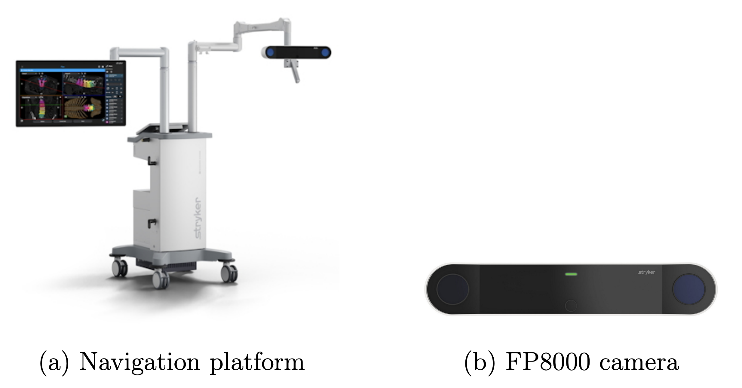
Accurate tracking of surgical instruments is essential for both the success and safety of procedures. One of Stryker’s key navigation systems is the FP8000 camera system. It combines two near-infrared (NIR) cameras and a high-resolution RGB camera. The NIR cameras track passive fiducial markers via triangulation, providing real-time 3D coordinates, while the RGB camera captures high-resolution images of the surgical field.
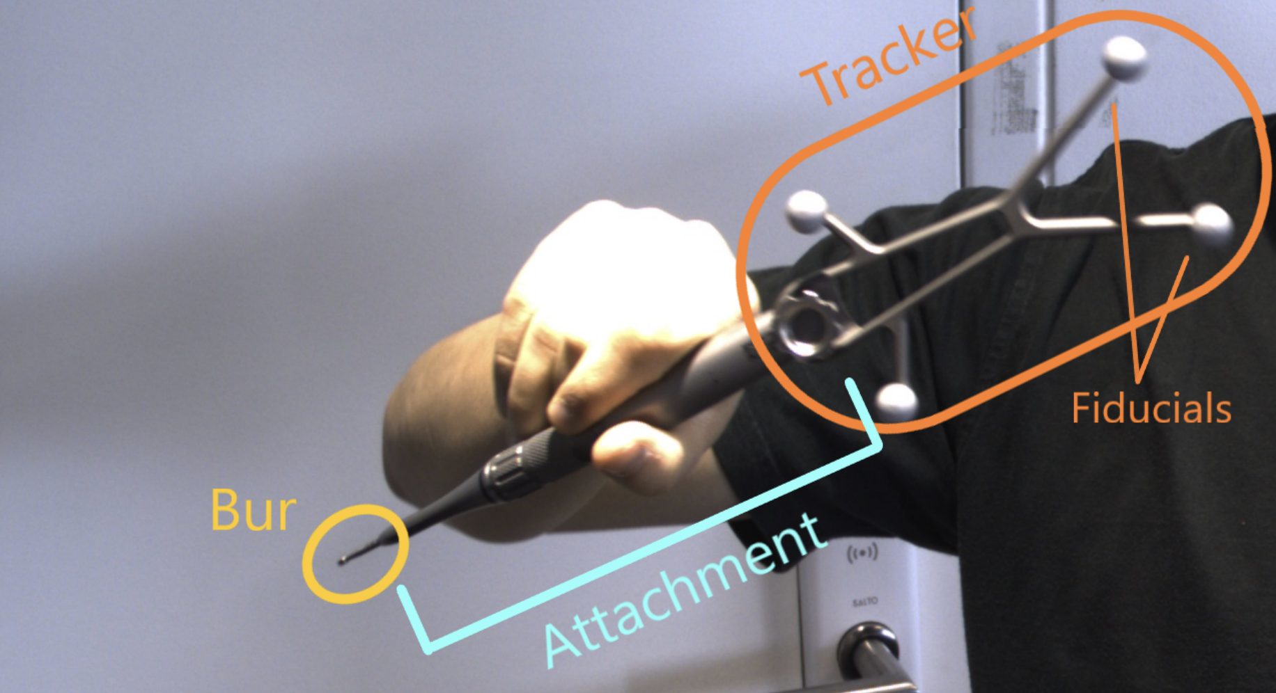
My internship focused on the High-Speed Drill (HSD) surgical tool. It is composed of:
- a tracker (with reflective fiducials),
- an attachment (straight or twisted),
- and the bur, the cutting or drilling head.
The existing workflow to track the HSD required manual calibration of each instrument to determine the precise 3D offset between the tracker and the bur tip. Since a surgery may involve dozens of instruments, and each calibration could take minutes, the setup process was inefficient and time-consuming.
The project therefore aimed to design a faster, video-based calibration pipeline using the RGB camera and deep learning. By automatically detecting keypoints on the tool and reconstructing the bur tip position in 3D, the goal was to minimize user effort while maintaining millimeter-level precision. This article is about how I implemented a 10-second video-based calibration pipeline reaching an average error of 3 mm.
Global Pipeline
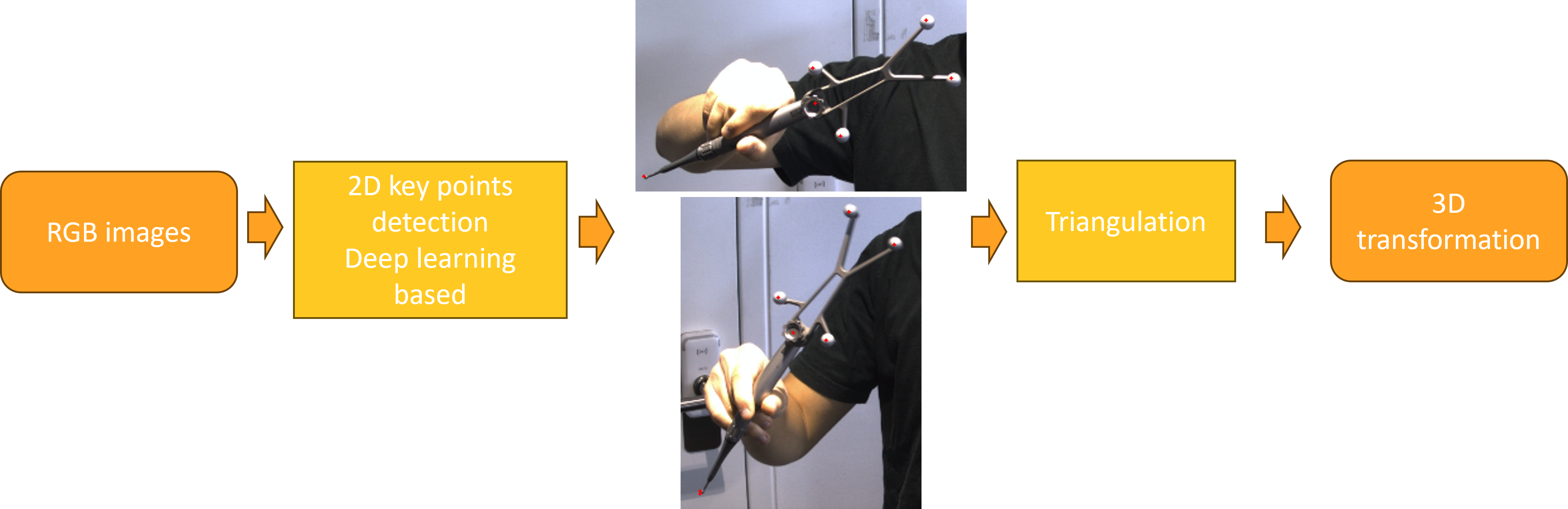
The idea was to replace manual calibration with a video-based deep learning approach.
At each video frame, the system already knows the 3D position of the tool’s tracker from the NIR cameras. The task of the neural network is to predict the 2D position of the bur tip in the RGB image.
By combining these two sources of information across many frames, the 3D geometry of the tool can be reconstructed through triangulation. Using even more frames makes the triangulation more robust, since errors in single-frame predictions can be averaged out.
This approach avoids the limits of end-to-end depth estimation which is not precise enough at the millimeter scale and requires huge amounts of annotated data. This two-step approach also make use of the existing manual calibration process to create a training dataset.
In short, the pipeline achieves precise calibration by merging:
- 2D tip predictions from a keypoint detection model,
- 3D tracker positions from the NIR system,
- and a multi-frame triangulation process to minimize errors.
Data Collection and Preparation
Building a reliable dataset was a key step of the project. The goal was to cover different tool attachments, burs, lighting conditions, and backgrounds so that the model could generalize well.
Data Acquisition
I collected the dataset directly with the FP8000 camera, obtaining:
- RGB images in real surgical-like conditions,
- 3D tracker positions from the navigation system,
- and the ground truth 3D transformations from manual calibration.
The 3D data was projected onto the 2D images using linear algebra transformations and OpenCV’s camera distortion parameters (radial, tangential, and prism coefficients).
Data Cleaning
To ensure quality:
- Blurry frames were discarded using a motion score derived from high-frequency tracker data (>300 Hz).
- Samples with poor tracker quality scores were removed.
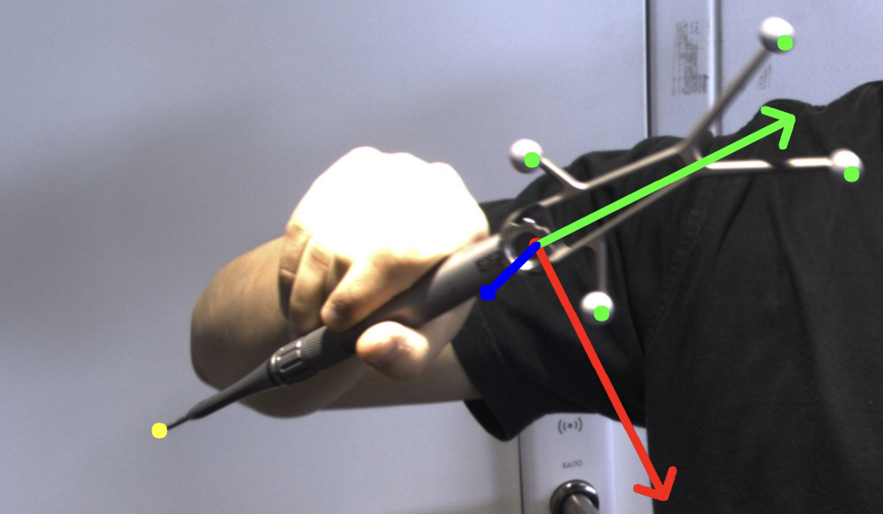
- Manual checks verified the seven annotated keypoints (four fiducials, tool center, bur center, and bur tip). Samples with <2-pixel error on the bur tip were kept.
The final dataset contained 1,047 training images and 645 test images.
Data Augmentation
To make the model robust, I applied random flips, rotations, brightness/contrast changes, and random cropping.
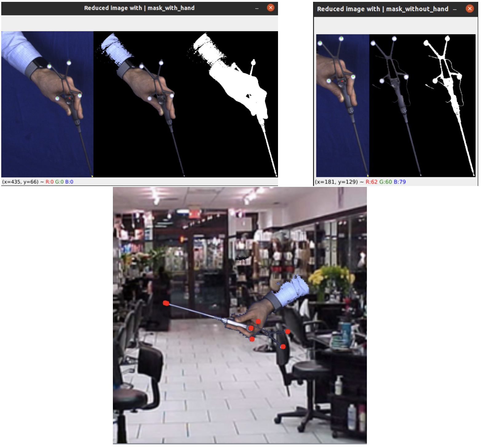
Additionally, I created synthetic data: tools were filmed against a blue drape, segmented with GrabCut, and then pasted onto random indoor backgrounds with rotation and scaling. This Photoshop augmentation helped simulate realistic variability.
HRNet Training
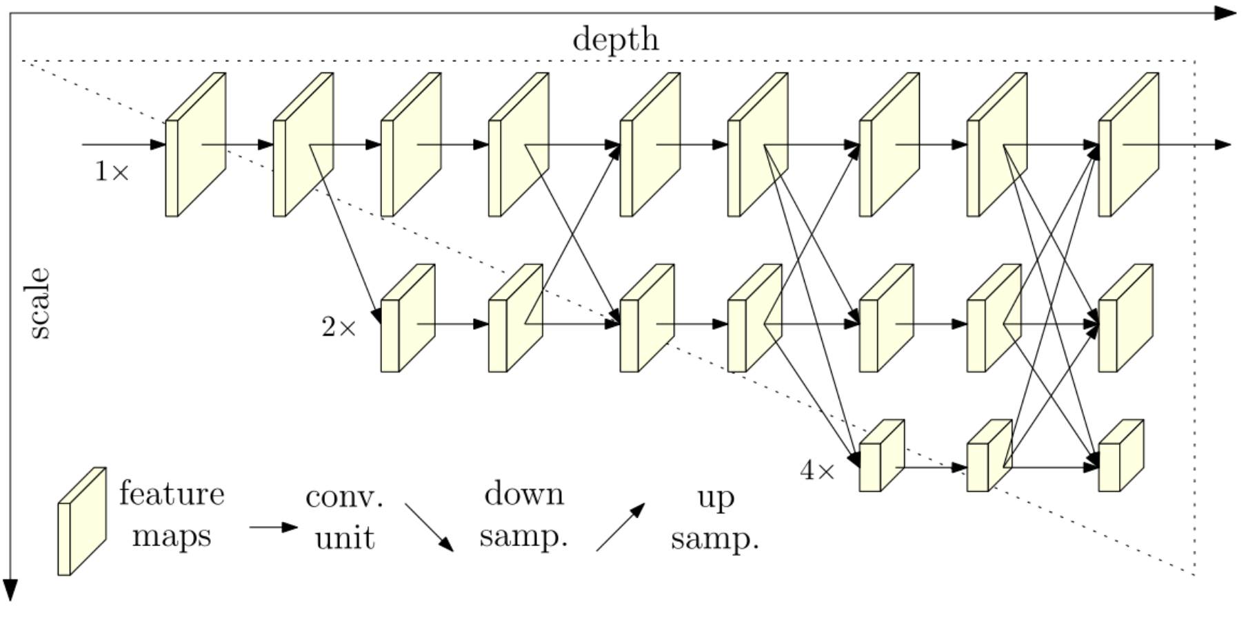
For detecting surgical tool keypoints, I used the HRNet architecture in PyTorch. Instead of training from scratch, I initialized the model with pretrained weights from human pose estimation, which gave faster convergence and better accuracy than random initialization.
The training objective was an MSE loss on Gaussian heatmaps centered around keypoints. I also used Online Hard Keypoint Mining (OHKM), putting more weights on hard samples. Then I added more weight to the tip keypoint since it was the most critical one.
On the data side, I found that mixing 2/5 synthetic images with real ones gave the best trade-off between generalization and stability. Data augmentation (rotations, brightness/contrast changes) significantly improved test performance, especially under challenging lighting.
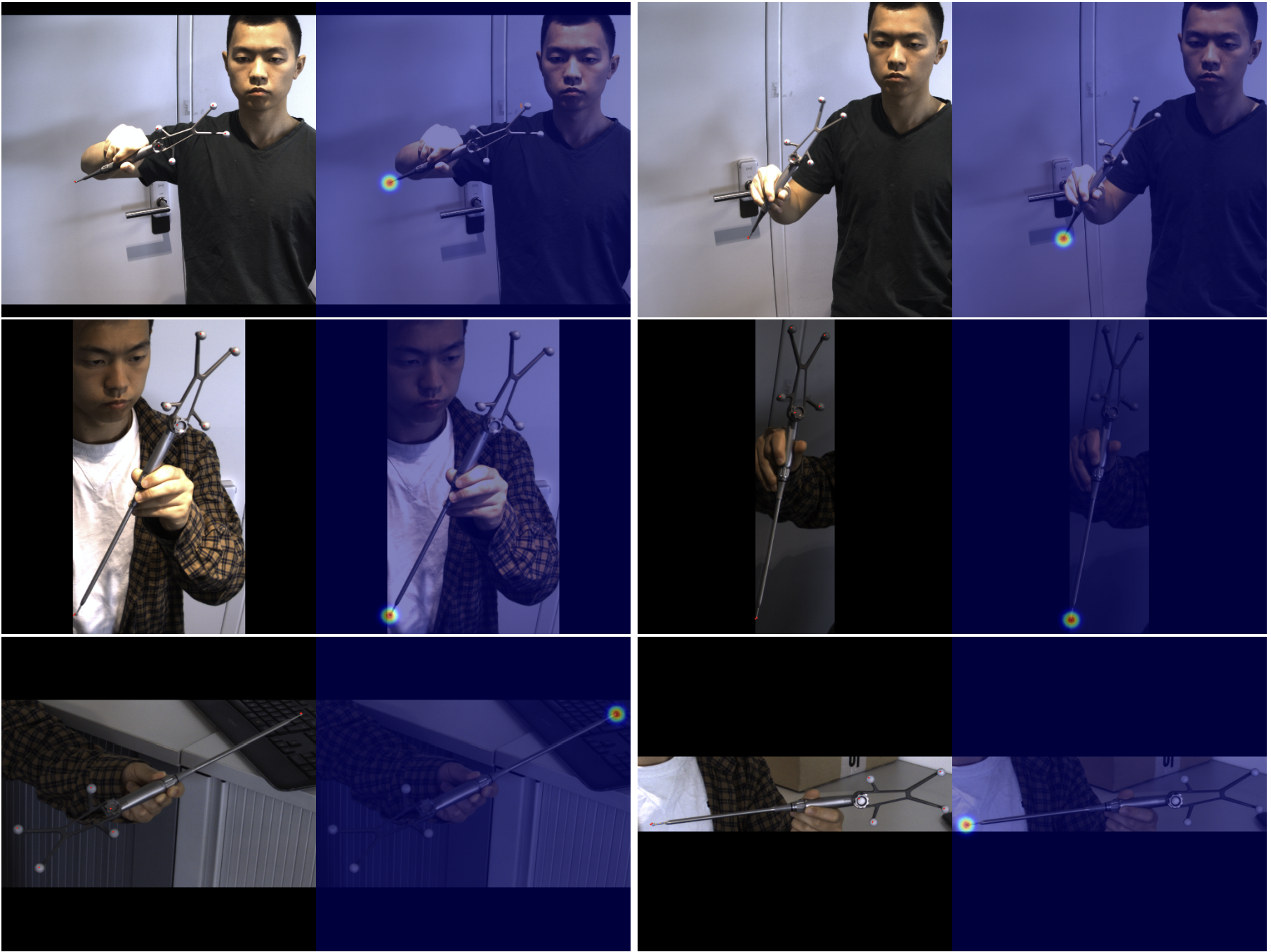
At inference, I applied multi-flip ensembling to reduce variance. Together with the refined loss functions, the final model achieved an MSE of ~2.6 pixels for the tip, which corresponds to sub-millimeter precision in real-world coordinates.
Random test results:
Triangulation of the Tip
The calibration problem can be framed as an inverse projection task. Normally, given the tracker’s 3D pose and the camera parameters, we can project the tool tip into the image. Here, we do the opposite: using the 2D keypoint predictions of the tip together with the known tracker positions, we estimate the 3D transformation from the tracker to the tip.
Each frame defines a 3D line on which the tip must lie. By collecting many frames, the final tip position can be computed as the point that minimizes the distance to all these lines, similar to multi-view triangulation, but using one RGB camera over time instead of multiple cameras.
Undistortion
A key preprocessing step was undistorting the images. I tested different distortion models and found that OpenCV’s implementation (which includes prism coefficients in addition to radial and tangential terms) achieved the best accuracy, with residual errors around 0.1 pixel after undistortion.
Constraints derivation from each frame
Then, everything else is linear algebra.
Let $F$ represent the intrinsic matrix of the camera, given by
\[F = \begin{bmatrix} f_x & 0 & c_x \\ 0 & f_y & c_y \\ 0 & 0 & 1 \end{bmatrix}\]- $T_c$ and $R_c$ denote the translation and rotation, respectively, of the tool center in the camera’s coordinate system.
- $t$ represents the unknown translation from the tool center to the tip of the tool.
According to projective geometry, we know that
\[\psi \begin{pmatrix}x\\y\\1\end{pmatrix} = F (T_c + R_c t)\]where $x$ and $y$ are the coordinates of the tip on the image, and $\psi$ is unknown.
By multiplying both sides by $\begin{pmatrix}0 & 0 & 1\end{pmatrix}$, we obtain
\[\psi = \begin{pmatrix}0 & 0 & 1\end{pmatrix}F (T_c + R_c t) = \begin{pmatrix}0 & 0 & 1\end{pmatrix} (T_c + R_c t)\]Let’s note
\[B = \begin{pmatrix} 0 & 0 & 1\\ 0 & 0 & 1\\ 0 & 0 & 1 \end{pmatrix}\]Therefore, we have
\[\psi \begin{pmatrix}1\\ 1\\ 1\end{pmatrix} = B (T_c + R_c t)\]Additionally, we consider
\[D =\begin{pmatrix}x & 0 & 0\\ 0 & y & 0\\ 0 & 0 & 1\end{pmatrix}\]Thus, we can express
\[\psi \begin{pmatrix}x\\ y\\ 1\end{pmatrix} = D \psi \begin{pmatrix}1\\ 1\\ 1\end{pmatrix} = D B (T_c +R_c t)\]By replacing this expression in the first equation, we obtain
\[DB(T_c + R_c t) = F(T_c+R_c t)\]As a result, we have
\[(DB-F) T_c + (DB - F) R_c t = 0\]It can be verified that the last row of $DB-F$ is always zero, meaning that we have exactly two non-zero equations. The other rows are non-zero since the diagonal of $DB-F$ is negative, ensuring that the rank is always 2.
Optimization Problem
For every image, these equations remain valid. As a result, when dealing with more than two images, we encounter an overdetermined problem. Each image provides a 3D line parametrized by the two equations. As the number of lines exceeds two, we can determine the optimal point by minimizing the L2 distance to all lines. This optimization problem is convex, allowing for a unique and analytically solvable solution.
Indeed, we can define
\[M = \begin{pmatrix} [(DB-F)R_c]_{1:2}\\ \vdots \\ \end{pmatrix}\] \[b = \begin{pmatrix}[(DB-F)T_c]_{1:2}\\ \vdots \\ \end{pmatrix}\]Here, $M$ is a $(2n, 3)$ matrix and $b$ is a $(2n, 1)$ vector.
It is important to note that all the matrices involved are in the world coordinate system, which differs from the camera coordinate system. Hence, it is necessary to use the following transformations:
\[R_c = R_{cam} R_{center}\] \[T_c = R_{cam} T_{center} + T_{cam}\]In an ideal scenario, we would have
\[Mt+b = 0\]The optimization problem aims to minimize $\left | Mt+b \right |^2$.
\[\nabla_t\left \| Mt+b \right \|^2 = 2 M^TMt + 2 M^T b = 0\]Solving this equation yields
\[t = - (M^TM)^{-1} M^T b\]The matrix $M^TM$ is a square symmetric non-negative matrix with a rank of at least 2. In practical scenarios, it is highly improbable for this matrix to be non-invertible. The condition for ensuring its invertibility is that the positions should not align on a 3D line from the camera’s perspective.
Results
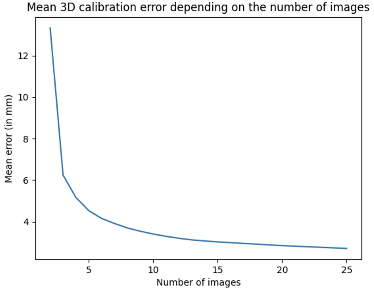
The method achieved an average error below 3.0 mm when using 25 frames (≈10 seconds of video before filtering). Considering that the manual calibration used as ground truth can itself deviate by up to 2 mm, this level of accuracy is very strong and demonstrates the effectiveness of the approach.
Thoughts
This project marked a significant milestone in my deep learning journey. Deep learning is not only about training models and optimizing them, it is about understanding how to use them. It is very unlikely that Deep learning will give the solution end-to-end, but it is very likely that it will give the solution to a part of the problem. After this internship, I realized that my math skills can solve so many problems that I never thought I could solve.
If you want more details, you can check the complete report.
-
Previous
Photogen AI - Founding a Startup on Diffusion Models -
Next
Analyzing Business Opportunities at Etandex