Training a Foundation Model for EEG Time Series at Beacon Biosignals

Project Overview

This work was conducted during my Master’s thesis internship at Beacon Biosignals, an American company developing healthcare solutions for analyzing brain activity. My research focused on training a foundation model for sleep EEG time series using self-supervised learning (SSL). I adapted contrastive learning and DINO from the computer vision literature to EEG data.

Because the project is closed-source, I cannot disclose specific data or implementation details. Instead, this article outlines the scientific motivation, relevant literature, and the conceptual approach that guided the work.

Summary

Electroencephalography (EEG) is a non-invasive method used to record the brain’s electrical activity through electrodes placed on the scalp. It plays a central role in understanding brain dynamics and diagnosing sleep disorders. However, large-scale annotation of EEG data is costly and time-consuming, as it requires expert clinicians to score hours of recordings.

This limitation motivates the development of an EEG foundation model: a large pretrained model that learns rich representations from vast amounts of unlabeled data and can later be fine-tuned for specific tasks such as sleep staging or pathology detection.

Inspired by recent progress in computer vision and natural language processing, we designed and trained EEG encoders able to capture both temporal and spatial information across channels. In downstream sleep stage classification, the pretrained model reaches within 3% of the performance of fully supervised models, while being trained on only 5% of the annotated data.

Motivation and Objectives

At Beacon, foundation models serve two main goals. First, they accelerate the development of specialized models by providing strong pretrained backbones that require minimal labeled data for fine-tuning. Second, they generate meaningful latent representations that help researchers explore, visualize, and interpret EEG data more effectively.

Training such a model requires balancing generalization and transferability. A foundation model must not only perform well on the data it has seen, but also adapt effectively to new subjects, devices, or even recording conditions. This paradigm, already dominant in language and vision [36, 37, 38], is still emerging in neuroscience, where signal variability and noise make it particularly challenging.

A bit of Literature

Sleep Staging

Sleep staging is the most studied problem on EEG data and serves as a key benchmark for evaluating new architectures. Early systems relied on handcrafted features: frequency bands, spectral power, or temporal dynamics, processed by traditional machine learning algorithms such as linear regression [1], decision trees [2], or ensemble models [3]. These approaches offered interpretability but struggled with generalization.

The rise of deep learning introduced more robust end-to-end methods. DeepSleepNet [5] and SeqSleepNet [6] combined convolutional and recurrent layers to capture local and sequential dependencies, while U-Sleep [8], inspired by the U-Net architecture [7], achieved strong results through multi-scale feature extraction. Later, RobustSleepNet [9] improved adaptability by integrating attention mechanisms across EEG channels, allowing the model to handle varying electrode configurations.

Annotation quality is a key challenge: sleep scoring is inherently subjective, with inter-clinician variability affecting the reliability of labels [10]. Datasets annotated by multiple experts and aggregated via majority voting have become standard to mitigate this issue. On such benchmarks, state-of-the-art models typically achieve 85–90% accuracy, setting a realistic upper bound for current methods.

Representation Learning for Time Series

While self-supervised learning has transformed vision and language, its application to time series and particularly to EEG remains relatively recent. Banville et al. [11] introduced one of the earliest SSL tasks for EEG, training models to infer temporal relationships between signal segments. Mohsenvand et al. [12] explored contrastive learning on single channels, showing that channel-specific encoders can capture useful representations when later combined. Thapa et al. [13] extended this idea to multi-modal signals, including EEG, ECG, and respiration, through joint contrastive objectives.

Transformers have also begun to shape this domain. Eldele et al. [14] and Das et al. [15] demonstrated the advantages of masked or autoregressive transformer training for time series, while Neuro-GPT [16] explored a decoder-only transformer tailored for EEG. Some studies [17, 18] have highlighted that generative losses are less effective on EEG, recommending representation-based objectives like contrastive or distillation losses instead, due to the signal’s inherently low signal-to-noise ratio.

Lessons from Computer Vision

The computer vision community has pioneered many of the methods for representation learning. Self-supervised representation learning in images began with contrastive methods like SimCLR [20], PIRL [21], and MoCo [22], where models learn to bring augmented views of the same image closer in the embedding space. Subsequent approaches such as BYOL [23] and DINO [24] refined this paradigm by removing negative samples and leveraging teacher-student architectures, stabilizing training and improving scalability.

Multi-modal extensions like CLIP [19] demonstrated that large-scale contrastive training can yield semantically aligned embeddings across different data types, bridging modalities like image and text. These works underpin modern DINOv2 [25] and other large vision transformers, offering valuable insights into how similar architectures might be leveraged for EEG data, where multiple channels act as spatial dimensions and temporal structure mirrors sequential dependencies in video.

Scaling and Efficiency

A recurring lesson across modalities is that scale drives performance. Studies on scaling laws in language [31], vision [32], and image-text contrastive models [33] have shown that model capacity, dataset size, and compute power follow predictable relationships. Larger models are not only more accurate but also more sample-efficient: they learn faster from limited labeled data. For EEG, where annotated datasets are inherently small, this principle is particularly relevant: a well-pretrained large model may drastically reduce the need for human scoring.

Method

Architectures

BIOT [18] extends the Transformer architecture to time series analysis.
We reimplemented the BIOT encoder for classification, following a design analogous to the Vision Transformer (ViT), but adapted to multi-channel EEG data.

We adopt the tokenization pipeline from BIOT, which transforms a raw EEG segment into a sequence of spatio-spectral tokens:

Resampling: Each EEG signal is resampled to $100\,\text{Hz}$, yielding data of shape $\mathbf{X} \in \mathbb{R}^{N_c \times T},$ where $N_c$ is the number of channels and $T$ the temporal length.
Fourier Transform: A short-time Fourier transform (STFT) with $50\%$ overlap is applied to convert the signal into the frequency domain: $\mathbf{X}_f \in \mathbb{R}^{N_c \times T' \times N_f}$ where $T’$ is the number of time bins (each representing a 1-second window) and $N_f$ the number of frequency bins.
Frequency Projection: A fully connected layer operates along the frequency axis to embed spectral information into a latent space: $\mathbf{Z} = \text{FC}(\mathbf{X}_f) \in \mathbb{R}^{N_c \times T' \times n_{\text{hid}}}$ where $n_{\text{hid}}$ is the hidden dimensionality.
Channel Embedding: Each EEG channel receives a learned embedding vector $\mathbf{e}_c$, added to its corresponding sequence tokens to encode spatial identity.
Positional Encoding: Temporal order is preserved by adding sinusoidal or learned positional encodings $\mathbf{p}_t$.
Flattening: The resulting tensor is reshaped into $\mathbf{Z}' \in \mathbb{R}^{(N_c \cdot T') \times n_{\text{hid}}}$ forming the input token sequence for the Transformer.

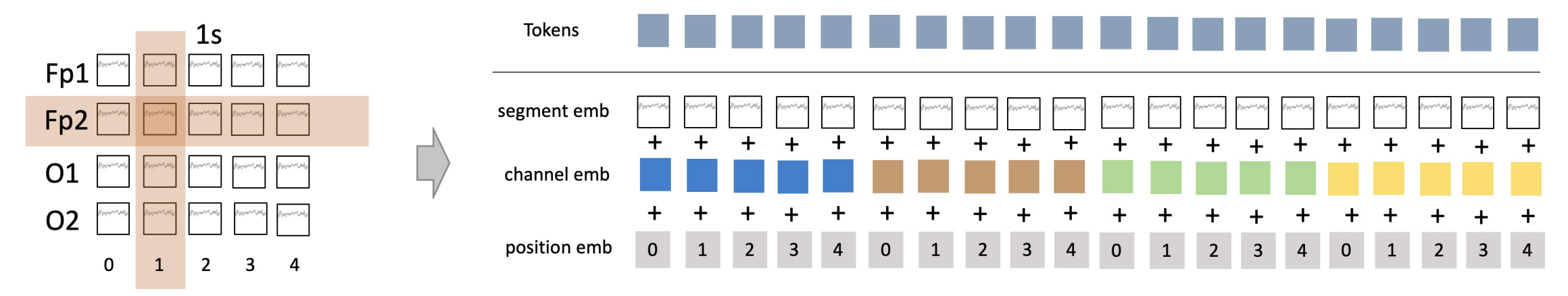
A learnable [CLS] token is prepended to the sequence, and the data is passed through an encoder-only Transformer. The final hidden state corresponding to the [CLS] token, denoted $\mathbf{h}_{\text{CLS}}$, serves as the representation of the entire EEG segment for downstream classification tasks.

Contrastive Learning

Contrastive learning is a self-supervised framework that aims to learn representations by distinguishing between similar and dissimilar pairs of data. The central idea is to bring positive pairs closer in the embedding space while pushing negative pairs farther apart. Positive pairs are generated from a single time series chunk on which we apply two different augmentations. By doing so, the model learns meaningful and invariant features without relying on explicit labels, which is particularly valuable in settings like EEG analysis where annotated data is scarce.

Prior work [22, 23] suggests that contrastive learning is better suited for EEG signals than masked pretraining. While masked pretraining focuses on predicting missing segments, the high noise level in EEG makes it difficult to infer meaningful content from partially observed signals. Contrastive methods instead optimize for consistency between different augmented views of the same input, effectively learning invariant and discriminative representations. This approach can thus be viewed as an adaptation of masked pretraining that bypasses its limitations in noisy physiological data.

The contrastive framework defines a family of transformations $\mathcal{T}$ that produce distinct but semantically consistent views of an input $x$. From $x$, two transformed samples $x^i, x^j \sim \mathcal{T}(x)$ form a positive pair.
An encoder $f$ followed by a projection head $g$ maps them to latent representations:

\[z_i = g(f(x^i)), \quad z_j = g(f(x^j))\]

The model is trained to maximize the cosine similarity between $z_i$ and $z_j$, while minimizing similarity to representations of other samples in the batch.

This objective is implemented using the Information Noise-Contrastive Estimation (InfoNCE) loss, which can be expressed as:

\[L = - \sum_{k=1}^{n} \log \frac{\exp(\text{sim}(z^{(k)}_i, z^{(k)}_j)/\tau)} {\sum_{l=1}^{n} \exp(\text{sim}(z^{(k)}_i, z^{(l)}_j)/\tau)},\]

where:

\[\text{sim}(z^{(k)}_i, z^{(l)}_j) = \frac{z^{(k)}_i \cdot z^{(l)}_j}{\|z^{(k)}_i\| \, \|z^{(l)}_j\|}.\]

Here, $\tau$ is a temperature parameter that controls how sharply similarities are weighted.

The numerator enforces high similarity between the positive pair $ (z^{(k)}_i, z^{(k)}_j) $.
The denominator aggregates similarities with all other representations in the batch, penalizing high similarity to negatives.

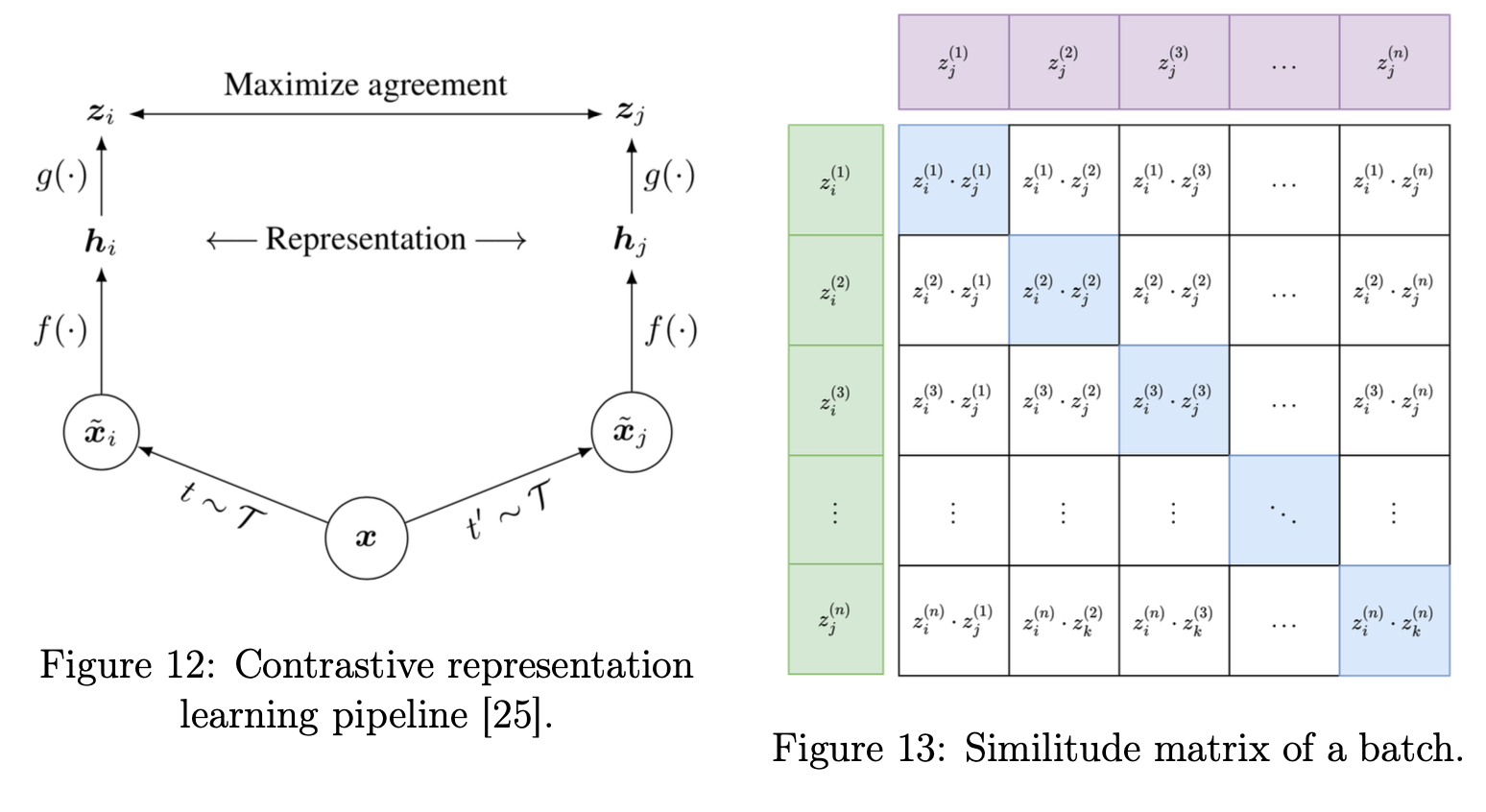
From a probabilistic perspective, InfoNCE performs an $n$-way classification task, where each sample acts as its own class. The similarity matrix serves as the set of logits for this implicit classification.
For a batch of size $n$, there are $n$ positive pairs and $n(n-1)$ negative pairs, making the task increasingly challenging and potentially more robust as batch size grows.

DINO

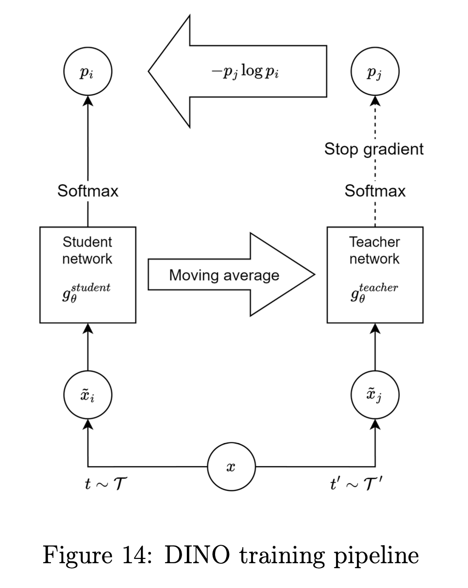
DINO (Distillation with No Labels) [24, 25] is a self-supervised learning framework originally introduced for computer vision tasks. It learns meaningful representations without requiring labeled data and can be viewed as a natural evolution of contrastive learning. By leveraging a teacher–student distillation mechanism, DINO eliminates the need for explicit negative pairs or large batch sizes, which are key bottlenecks in contrastive methods.

DINO integrates several ideas from recent advances in self-supervised learning that specifically address the weaknesses of contrastive learning. Traditional contrastive methods rely on a large number of negative pairs to prevent feature collapse, which often requires large batch sizes and significant memory resources. DINO bypasses this constraint through self-distillation: the model learns from its own progressively refined representations.

Moreover, DINO has proven effective at simultaneously capturing local and global contextual information. This is particularly valuable for EEG signals, where both transient, high-frequency patterns (local) and slower brain rhythms or long-term dependencies (global) play critical roles in downstream tasks such as sleep staging or pathology detection. These properties make DINO a compelling alternative to contrastive pretraining for time-series foundation models.

DINO relies on a teacher–student setup. Both networks share the same architecture (e.g., a Transformer encoder), but the teacher’s weights evolve as an exponential moving average (EMA) of the student’s parameters.

We define two families of augmentations:

Global transformations $\mathcal{T}^{\text{glob}}$: produce large-scale crops (e.g., covering >50% of the temporal signal);
Local transformations $\mathcal{T}^{\text{local}}$: produce smaller crops (<50% of the signal), emphasizing fine-grained temporal information.

Pseudo code for DINO:

Input:

Student and teacher networks: $g_s, g_t$
Teacher momentum rate: $\lambda$

Initialization:
$g_t.\text{params} = g_s.\text{params}$

for x in loader:  # Load a minibatch x with n samples
    # Generate random views (global/local)
    x_glob_i, x_loc_i = t_glob(x), t_loc(x)       # Student views
    x_glob_j = t_glob(x)                          # Teacher view

    # Forward pass
    z_glob_i, z_loc_i = gs(x_glob_i), gs(x_loc_i) # Student outputs
    z_glob_j = SKC(gt(x_glob_j))                  # Teacher output with SK centering

    # Stop gradient for the teacher
    z_glob_j = z_glob_j.detach()

    # Compute local and global losses
    loss_loc  = CrossEntropy(z_glob_j, z_loc_i)
    loss_glob = CrossEntropy(z_glob_j, z_glob_i)

    # Total loss
    loss = 0.5 * loss_loc + 0.5 * loss_glob
    loss.backward()  # Backpropagate through student

    # Update student and teacher
    update(gs)  # SGD update for student
    gt.params = λ * gt.params + (1 - λ) * gs.params  # Momentum update for teacher

Given a sample $x$, we generate one or more global views $x^j \in \mathcal{T}^{\text{glob}}(x)$ and local views $x^i \in \mathcal{T}^{\text{local}}(x)$.
The student and teacher networks output corresponding probability distributions: $p_i = \text{softmax}\left(\frac{z_i}{\tau_s}\right), \quad p_j = \text{stopgrad}\left(\text{softmax}\left(\frac{\text{center}(z_j)}{\tau_t}\right)\right),$ where $\tau_s$ and $\tau_t$ are temperature parameters for the student and teacher, respectively.

A centering operation is applied to the teacher’s output before the softmax to avoid representational collapse. This step ensures that the teacher’s output distribution maintains diversity, often implemented through a variant of Sinkhorn-Knopp normalization [25].

The loss function is a cross-entropy between the teacher’s and student’s distributions: $\mathcal{L}_{\text{DINO}} = - \sum_{k} p_j^{(k)} \log p_i^{(k)}.$

Only the student branch is updated via backpropagation, while the teacher is updated using EMA: $\theta_{\text{teacher}} \leftarrow \lambda \, \theta_{\text{teacher}} + (1 - \lambda) \, \theta_{\text{student}},$ where $\lambda$ is the momentum coefficient (typically between 0.9 and 0.9995).

This asymmetric design combining stop-gradient, centering, and EMA updates prevents collapse and enables stable training without requiring explicit negative samples.

In summary, DINO provides a scalable, noise-resilient, and label-free training strategy for EEG data, capable of capturing hierarchical temporal features and long-range dependencies efficiently.

Conclusion

This project explored how self-supervised learning can be adapted to EEG to train large-scale, general-purpose foundation models. By extending contrastive and distillation-based methods like SimCLR and DINO to time series, we showed that unlabeled EEG recordings can yield rich, transferable representations that approach supervised performance with minimal labels.

Interestingly, the most difficult parts of the project were not the algorithms themselves but the infrastructure and scaling. A large portion of my time was spent debugging pipelines, optimizing preprocessing, and tuning distributed training setups. In many ways, the project was as much about engineering deep learning systems at scale as about research.

References

[1] Christian Berthomier et al. Automatic analysis of single-channel sleep EEG: validation in healthy individuals. Sleep, 30(11):1587–1595, 2007.

[2] Tarek Lajnef et al. Learning machines and sleeping brains: Automatic sleep stage classification using decision-tree multi-class support vector machines. Journal of Neuroscience Methods, 250:94–105, 2015.

[3] Jeroen Van Der Donckt et al. Do not sleep on traditional machine learning: Simple and interpretable techniques are competitive to deep learning for sleep scoring. Biomedical Signal Processing and Control, 81:104429, 2023.

[4] Stanislas Chambon et al. A deep learning architecture for temporal sleep stage classification using multivariate and multimodal time series. IEEE Transactions on Neural Systems and Rehabilitation Engineering, 26(4):758–769, 2018.

[5] Akara Supratak et al. DeepSleepNet: A model for automatic sleep stage scoring based on raw single-channel EEG. IEEE Transactions on Neural Systems and Rehabilitation Engineering, 25(11):1998–2008, 2017.

[6] Huy Phan et al. SeqSleepNet: End-to-end hierarchical recurrent neural network for sequence-to-sequence automatic sleep staging. IEEE Transactions on Neural Systems and Rehabilitation Engineering, 27(3):400–410, 2019.

[7] Olaf Ronneberger, Philipp Fischer, and Thomas Brox. U-Net: Convolutional networks for biomedical image segmentation. MICCAI, 2015.

[8] Mathias Perslev et al. U-Sleep: Resilient high-frequency sleep staging. NPJ Digital Medicine, 4(1):72, 2021.

[9] Antoine Guillot and Valentin Thorey. RobustSleepNet: Transfer learning for automated sleep staging at scale. IEEE Transactions on Neural Systems and Rehabilitation Engineering, 29:1441–1451, 2021.

[10] Antoine Guillot et al. Dreem open datasets: Multi-scored sleep datasets to compare human and automated sleep staging. IEEE Transactions on Neural Systems and Rehabilitation Engineering, 28(9):1955–1965, 2020.

[11] Hubert Banville et al. Uncovering the structure of clinical EEG signals with self-supervised learning. Journal of Neural Engineering, 18(4):046020, 2021.

[12] Mostafa Neo Mohsenvand et al. Contrastive representation learning for electroencephalogram classification. ML4H, 2020.

[13] Rahul Thapa et al. SleepFM: Multi-modal representation learning for sleep across brain activity, ECG and respiratory signals. arXiv preprint arXiv:2405.17766, 2024.

[14] Emadeldeen Eldele et al. Self-supervised contrastive representation learning for semi-supervised time-series classification. IEEE TPAMI, 2023.

[15] Abhimanyu Das et al. A decoder-only foundation model for time-series forecasting. arXiv preprint arXiv:2310.10688, 2023.

[16] Wenhui Cui et al. Neuro-GPT: Developing a foundation model for EEG. arXiv preprint arXiv:2311.03764, 2023.

[17] Navid Mohammadi Foumani et al. EEG2Rep: Enhancing self-supervised EEG representation through informative masked inputs. arXiv preprint arXiv:2402.17772, 2024.

[18] Chaoqi Yang, M. Brandon Westover, and Jimeng Sun. BIOT: Cross-data biosignal learning in the wild. arXiv preprint arXiv:2305.10351, 2023.

[19] Alec Radford et al. Learning transferable visual models from natural language supervision. ICML, 2021.

[20] Ting Chen et al. A simple framework for contrastive learning of visual representations. ICML, 2020.

[21] Ishan Misra and Laurens van der Maaten. Self-supervised learning of pretext-invariant representations. CVPR, 2020.

[22] Kaiming He et al. Momentum contrast for unsupervised visual representation learning. CVPR, 2020.

[23] Jean-Bastien Grill et al. Bootstrap Your Own Latent (BYOL): A new approach to self-supervised learning. NeurIPS, 2020.

[24] Mathilde Caron et al. Emerging properties in self-supervised vision transformers. ICCV, 2021.

[25] Maxime Oquab et al. DINOv2: Learning robust visual features without supervision. arXiv preprint arXiv:2304.07193, 2023.

[26] Tongzhou Wang and Phillip Isola. Understanding contrastive representation learning through alignment and uniformity on the hypersphere. ICML, 2020.

[27] Xianghong Fang et al. Rethinking the uniformity metric in self-supervised learning. arXiv preprint arXiv:2403.00642, 2024.

[28] Young-Jin Park et al. Quantifying representation reliability in self-supervised learning models. arXiv preprint arXiv:2306.00206, 2023.

[29] Quentin Garrido et al. RankMe: Assessing the downstream performance of pretrained self-supervised representations by their rank. ICML, 2023.

[30] Vimal Thilak et al. LiDAR: Sensing linear probing performance in joint embedding SSL architectures. arXiv preprint arXiv:2312.04000, 2023.

[31] Jared Kaplan et al. Scaling laws for neural language models. arXiv preprint arXiv:2001.08361, 2020.

[32] Xiaohua Zhai et al. Scaling Vision Transformers. CVPR, 2022.

[33] Mehdi Cherti et al. Reproducible scaling laws for contrastive language–image learning. CVPR, 2023.

Training a Foundation Model for EEG Time Series at Beacon Biosignals ⭐ ⭐

Self-Supervised Learning for Sleep EEG Analysis with 95% Fewer Labels