Decoding Mouse Maze Position from Brain Signals

Last weekend I took part in Hacktion Potential, a 48-hour computational neuroscience hackathon at the Institut du Cerveau in Paris. Our team worked on decoding mouse maze position from brain signals: mapping high-dimensional neural activity to the (x,y) position of a mouse in a closed environment.

The hackathon goal was to design a decoding method that takes raw hippocampal data (spike activity recorded at ~20 kHz) and predicts spatial location.

Trajectory

Technical story

Since we had very limited time, we kept the approach simple: 1D-CNNs, a few ablations, and a focus on understanding the data and evaluation (splits, window size) rather than pushing state-of-the-art architectures.

Data

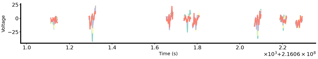
Recordings come from the hippocampus with a silicon probe at 20 kHz. Each probe has several shanks recording from different locations. For each decoding timepoint we have the true (x,y) position (sampled at ~15 Hz). Only timepoints where the mouse is moving are used for decoding, since position encoding is physiologically only relevant during movement.

The dataset is built from highpass-filtered, spike-focused activity. For each shank we: detect spikes when voltage exceeds 3× standard deviation on any channel.

Spike visualization

Model architecture and data ablation

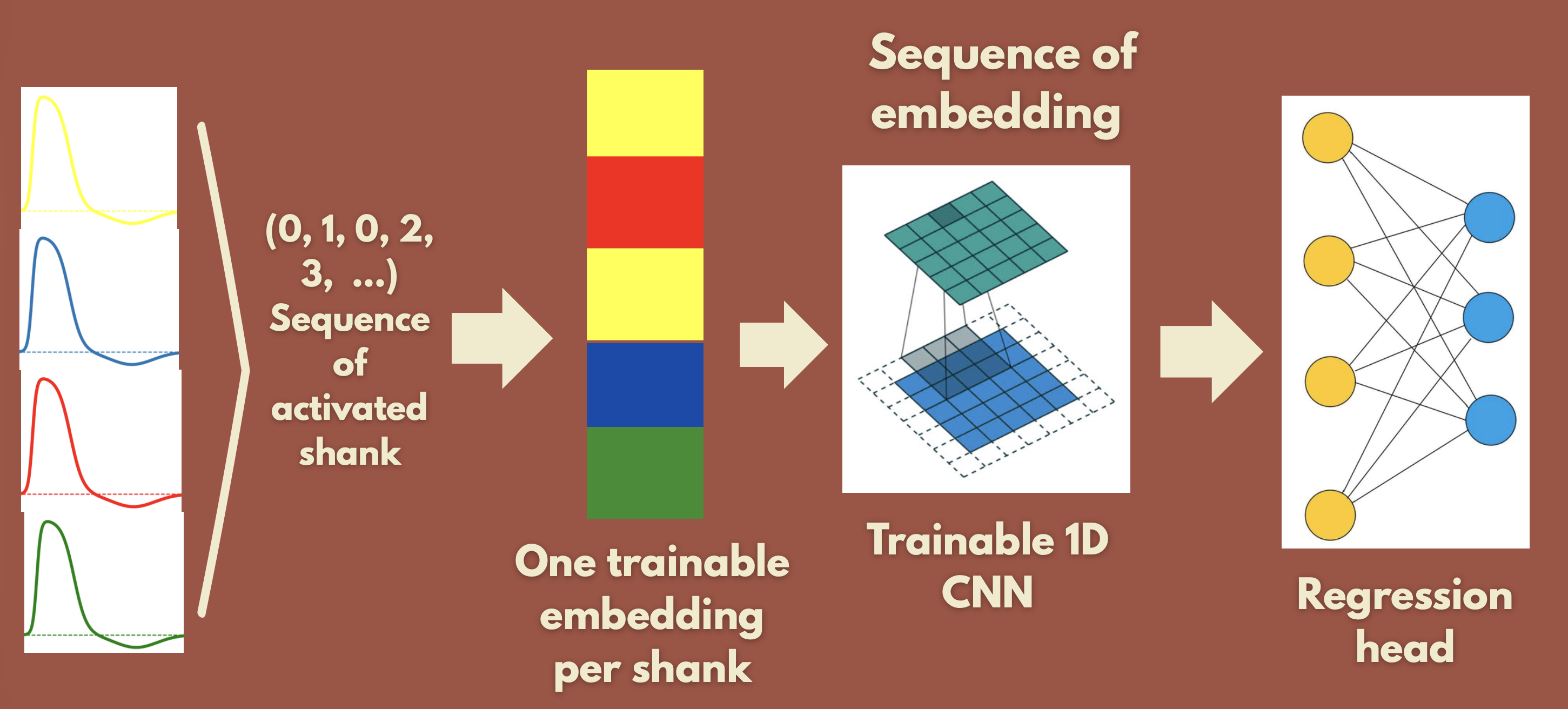
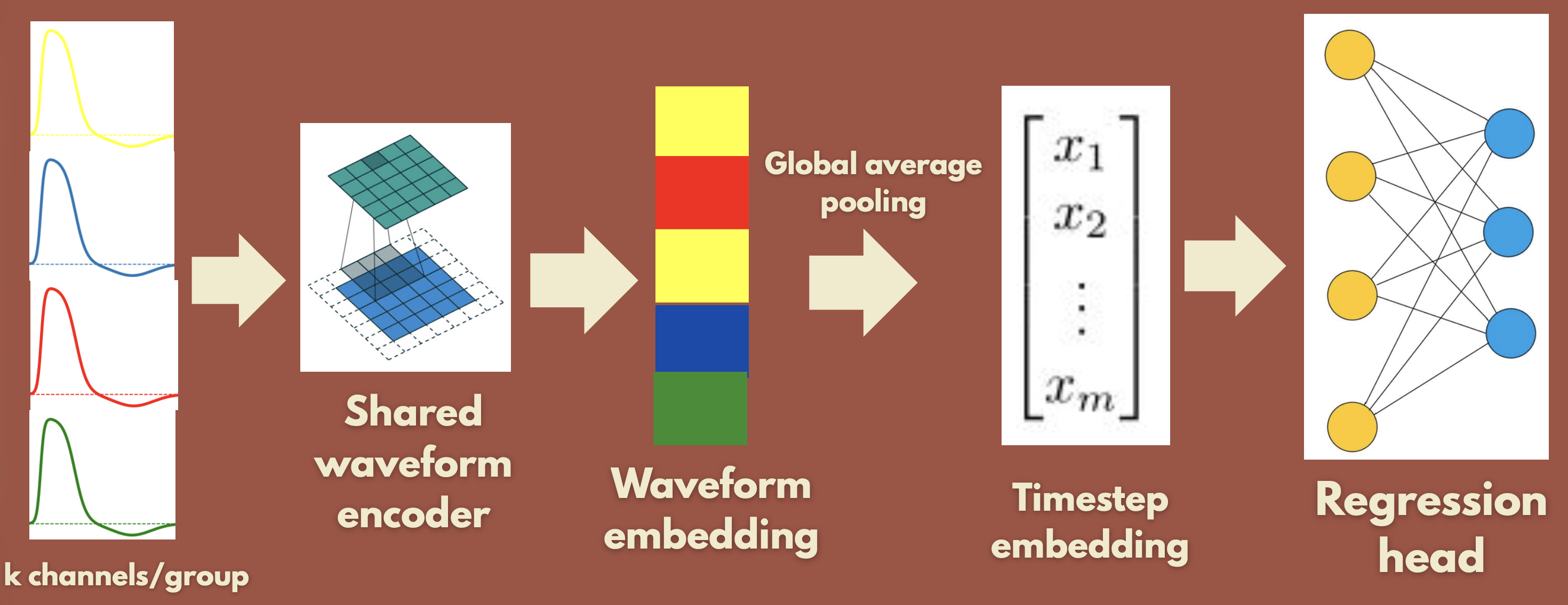
We tested whether spike waveforms are needed for decoding. Two models:

Spiking Embedding Network: only the sequence of spike indices (which shank fired). Trainable embeddings per shank → sequence → 1D-CNN → FC → (x,y).
Waveform Network: 1D-CNN on the actual waveforms, then global average pooling over the sequence → FC → (x,y).

Losses Spiking Embedding Network — Spiking Embedding — train vs test loss

Losses Waveform Network — Waveform — train vs test loss

Result: the Spiking Embedding Network does not generalize (low train loss, high test loss). The Waveform Network generalizes well. So waveform information appears necessary, likely because it identifies which neuron fired, not only when. All of this was with a random train/test split.

Window size

We varied the spike window length (18+18, 54+54, 126+126 timesteps around the peak), i.e. 36, 108, and 252 timesteps. All settings learn: 108 converged fastest, consistent with a trade-off between information and noise.

Below we show learning curves for both shuffled and temporal splits (split types are detailed in the next section).

Window 36 shuffled — Shuffled, window 36

Window 108 shuffled — Shuffled, window 108

Window 252 shuffled — Shuffled, window 252

Window 36 temporal — Temporal, window 36

Temporal split, window 108 — Temporal, window 108

Temporal split, window 252 — Temporal, window 252

Splitting issues

Train/test split had a large impact. We compared:

Temporal: train on first 90%, test on last 10% (as suggested).
Middle: test on middle 10%, train on the rest.
Shuffled: random split.

Split type	Lowest train MSE	Lowest test MSE
Temporal	0.018	0.103
Middle	0.030	0.081
Shuffled	0.036	0.054

Here, we did not use a validation set since we did not even tune hyperparameters.

Temporal and middle splits generalize poorly while shuffled seems to generalize better. That suggests that there might be distribution shift or non-stationarity over the session. Another hypothesis is that the data might not carry position information. However, that goes against the results of this study: Zhang, K. et al. (1998) ‘Interpreting Neuronal Population Activity by Reconstruction: Unified Framework With Application to Hippocampal Place Cells’, Journal of Neurophysiology, 79(2), pp. 1017–1044. We might also have some data leakage issues for the shuffled split.

Prediction visualization — Predictions on test (middle split)

Predictions on the test set are noisy but follow the trajectory. Notice that the model often predicts positions outside the maze.

Future directions

Model: tune hyperparameters, regularization, data augmentation, cleaner preprocessing to reduce overfitting and shift.
Generalization: run on multiple mice (current runs are one mouse).
Multi-subject: train on pooled data across mice.
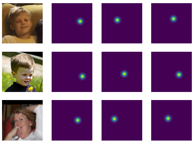
Model redesign: condition on maze geometry (e.g. ControlNet-style), predict position as a heatmap (example below), or add past positions as input.

Key points detection heatmaps — Example of predicting position as a heatmap (keypoint detection target).

Conclusion

We didn’t win, and the experiments weren’t really conclusive. I still really enjoyed the hackathon. The subject is really interesting and I got to get a glimpse back into neuroscience. I loved the opportunity to work at that pace. The experience was very stimulating.

Repository: github.com/clementw168/mouse-maze-position-from-brain-signals
Slides: presentation.pdf in the repo

A 48-hour proof of concept at Hacktion Potential