Take a graph $G$ and swap the roles of its vertices and edges: every edge becomes a node, and two of these nodes are linked whenever the edges they came from used to share an endpoint. That’s the line graph $L(G)$. It sounds like a cheap notational trick, but it turns out to be a real change of perspective: a lot of questions about the edges of $G$ become questions about the vertices of $L(G)$, where the standard vertex-level toolbox (coloring, cliques, GNN message passing…) applies directly.
This post is a tour through the theory of line graphs: how to define them, whether the map $G \mapsto L(G)$ can be undone, which graphs are line graphs, and where this shows up in machine learning. I’ll sketch the ideas, see the accompanying technical note for anyone who wants the details.
Definition and first example
\[V(L(G)) = E(G), \qquad e \sim f \iff e \cap f \neq \varnothing .\]Vertices of $L(G)$ are edges of $G$. Two of them are adjacent in $L(G)$ exactly when the corresponding edges of $G$ meet at a common vertex.
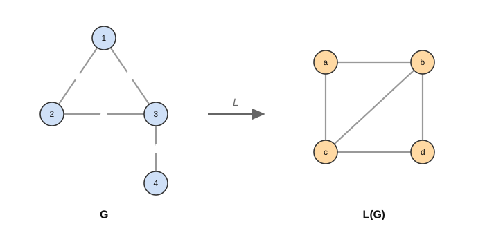
Edges $b$, $c$, $d$ all meet at vertex $3$ of $G$, so they form a triangle in $L(G)$. In general, every vertex $v$ of $G$ with degree $d_v$ contributes a clique of size $d_v$ to $L(G)$ (all the edges at $v$ are pairwise adjacent).
Two consequences fall out immediately: $L(G)$ has exactly $m = |E(G)|$ vertices, and an edge $e = uv$ has degree $d_u + d_v - 2$ in $L(G)$ (it shares $L(G)$-edges with the $d_u - 1$ other edges at $u$ and the $d_v - 1$ other edges at $v$). So an $r$-regular graph maps to a $(2r-2)$-regular one.
The three basic families
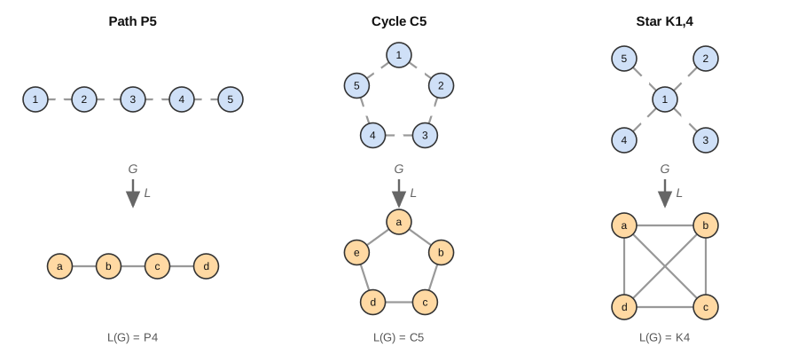
Paths shrink by one vertex, cycles are fixed points of the operator, and a star $K_{1,n}$ (all edges sharing one center) becomes a complete graph $K_n$, since all $n$ edges are pairwise adjacent. More generally, $L(K_n)$ is the triangular graph: its vertices are the pairs ${i,j}$, adjacent iff they intersect. $L(K_4)$ in particular is the octahedron.
Iterating $L$ almost always makes the graph bigger. Paths shrink and cycles stay put, but the moment some vertex has degree $\geq 3$, $L(G)$ already has more vertices than $G$, and the gap keeps widening under further iteration.
Can you undo it? Whitney’s theorem
Given only $L(G)$, can you recover $G$? The answer is yes, up to isomorphism, with only one exception in the entire universe of graphs.
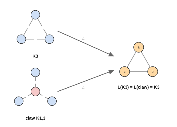
The triangle $K_3$ and the claw $K_{1,3}$ both have three edges that pairwise share an endpoint, so both map to $K_3$. These two graphs are not isomorphic, so the map $L$ is not injective in general but Whitney’s theorem (1932) says this is the only place injectivity fails:
Whitney’s theorem. For connected graphs $G, H$, $L(G) \cong L(H)$ implies $G \cong H$, unless ${G, H} = {K_3, K_{1,3}}$.
Every vertex $v$ of $G$ produces a clique $S_v \subseteq L(G)$ (the edges at $v$), and every vertex of $L(G)$, being an edge $uv$ of $G$, sits in exactly two such cliques, $S_u$ and $S_v$. So the cliques ${S_v}$ cover $L(G)$ with each vertex used exactly twice, and $G$ can be rebuilt by taking one point per clique and connecting two points whenever their cliques share a vertex of $L(G)$. This works perfectly as long as the $S_v$ are exactly the maximal cliques of $L(G)$. The only way that can fail is a triangle in $L(G)$ that could come either from three edges meeting at one vertex (a star, i.e. $S_v$ itself is that triangle) or from an actual triangle in $G$, precisely the $K_3$/claw coincidence. Outside that single case, the maximal cliques of $L(G)$ are unambiguous, and $G$ is determined.
Is every graph a line graph? No.
Consider the claw itself, $K_{1,3}$: could it be $L(G)$ for some $G$? Suppose it were. The center of the claw would be some edge $e = uv$, and the three leaves would be three edges of $G$, each touching $e$ (so each contains $u$ or $v$), but pairwise not adjacent. By pigeonhole, two of those three edges contain the same endpoint, say both contain $u$, but then they share $u$ and must be adjacent in $L(G)$, contradicting the claw’s structure. So no graph maps to the claw.
Because line graphs are closed under taking induced subgraphs (delete some edges of $G$ and their endpoints, and you get the line graph of what remains), this single fact propagates: any graph containing an induced claw is not a line graph. Being claw-free is necessary. It isn’t sufficient on its own, but three classical results sharpen it into an exact characterization:
- Krausz (1943): $H$ is a line graph iff its edges split into cliques such that every vertex of $H$ lies in at most two of them. (This is just ${S_v}$ from Whitney’s proof, read as a recipe instead of a certificate.)
- van Rooij–Wilf (1965): $H$ is a line graph iff it is claw-free and, whenever two triangles that are “odd” (some outside vertex sees exactly $1$ or $3$ of their corners) share an edge, the four vertices involved form a $K_4$.
- Beineke (1970): $H$ is a line graph iff it contains none of nine specific small graphs as an induced subgraph.
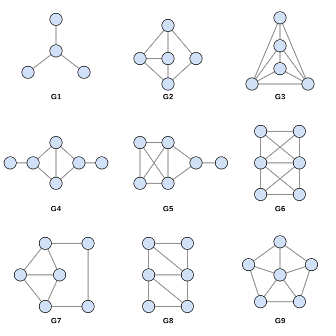
The existence of some finite forbidden list follows from the first two characterizations plus a locality argument: any minimal failure of the van Rooij–Wilf conditions is witnessed by a handful of vertices, so a minimal non-line-graph can’t be arbitrarily large. Pinning down that the list has exactly nine members, with at most six vertices each, took the explicit case analysis Beineke worked through. Therefore, checking for nine fixed small patterns is a polynomial-time test for “is this a line graph.”
Reconstructing the root graph
Krausz’s characterization directly constructs the $G$ from $L(G)$. If you can find the clique partition, you get $G$ for free: one vertex per clique, and each vertex of $H$ becomes the edge joining the (at most two) cliques it belongs to.
Two classical algorithms find that partition in linear time, $O(n+m)$, taking slightly different routes:
- Roussopoulos (1973) builds the partition incrementally: start from one edge of $H$, grow its clique using shared neighborhoods, and reject as soon as some Krausz invariant is violated (a vertex in three cliques, say).
- Lehot (1974) instead uses the van Rooij–Wilf local structure to read off candidate cliques vertex by vertex, assembles a tentative root graph $G$, and then verifies by recomputing $L(G)$ and comparing it to $H$.
Either way: recognizing a line graph and inverting it are the same problem, and both are as cheap as reading the input once.
Where line graphs show up in machine learning
Most GNNs pass messages between vertices. Plenty of interesting tasks are naturally about edges instead : will this link form, do these two edges belong to the same community, how do two interacting entities relate. Reading an edge-level answer out of a vertex-level GNN usually means pooling two endpoint embeddings together, which loses information. The line graph sidesteps this: since $V(L(G)) = E(G)$, an edge-level quantity on $G$ is already a vertex-level quantity on $L(G)$, so ordinary node classification machinery applies with no pooling step.
Link prediction. Cai, Li, Wang, and Ji (2021) extract a small subgraph around a candidate pair of vertices, take its line graph, and classify one specific vertex, the candidate link itself, directly, instead of scoring a pooled pair of node embeddings.
Community detection. Chen, Li, and Bruna (2019) augment message passing with the non-backtracking operator, a directed variant of the line-graph adjacency where an edge can’t immediately double back along itself, letting the network see edge-to-edge relationships a purely vertex-based GNN would miss.
ncRNA–protein interaction. Han and Zhang (2023, Computational and Structural Biotechnology Journal) use both levels together: an enclosing subgraph is extracted around a candidate ncRNA–protein pair, converted to its line graph so the pair becomes a single vertex again, and a graph attention network runs on top to make the final prediction.
Closing thought
The line graph is a nearly lossless change of perspective : Whitney’s theorem says it keeps essentially everything about $G$, and whenever a graph happens to be a line graph, a linear-time algorithm hands the root straight back. But that same fidelity is why it doesn’t compress: any vertex of degree three or more makes $L(G)$ bigger than $G$, not smaller. And exact inversion requires an exact line graph, which real data almost never gives you, repairing one into a line graph first is NP-complete. That’s probably why the machine-learning applications above all go one direction, from $G$ to $L(G)$, and never try to invert it. Whether a cheap approximate inverse could make this lossless view practically useful both ways is, as far as I know, still open.
For the fully rigorous version of this post with formal definitions, proofs, and the pseudocode for the inversion algorithms, see the accompanying technical note.